How Register Tokens Reshape Information Flow in Vision Transformers
Published:
Modern vision transformers like DINOv2 and DINOv3 include a curious architectural feature: register tokens — learnable vectors appended to the input sequence that participate in self-attention but correspond to no image region. Originally introduced to suppress attention artifacts, these tokens turn out to play a far more active role than their name suggests.
In this post, I walk through our findings from systematic token-zeroing experiments that reveal a double dissociation between CLS and register tokens, show that registers function as attention scaffolds rather than information stores, and trace the temporal dynamics of how register tokens acquire and sometimes release semantic content across network layers.
The DINO Family and the Register Problem
Self-supervised ViTs in 60 seconds
The DINO family of vision transformers learns visual representations through self-distillation — a student network learns to match the outputs of a momentum-updated teacher, without any labeled data. The result is a model whose internal representations capture rich semantic and spatial structure.
A standard ViT processes an image by splitting it into non-overlapping patches (typically 14×14 pixels), projecting each patch into an embedding, and prepending a learnable CLS token. All tokens — CLS plus patches — interact through self-attention across multiple transformer layers. At the output, the CLS token serves as a global image representation (useful for classification), while patch tokens retain spatial information (useful for segmentation and correspondence).

What do these patch features actually look like? The gallery below projects each model’s patch features into 3 PCA components (mapped to RGB). Notice how different models organize spatial information differently:
Interactive: PCA patch features
The artifact problem
Darcet et al. (2024) discovered that DINO and DINOv2 produce high-norm artifact tokens in low-information image regions — patches corresponding to sky, water, or uniform backgrounds would develop anomalously large activation norms that distorted downstream feature maps. Their solution: append 4 learnable register tokens to the input sequence. These registers participate in self-attention but are discarded at inference, absorbing the artifact computation and leaving patch tokens clean.
DINOv2 was then retrained with registers (DINOv2+reg), and the artifacts disappeared. But a question remained: what exactly are these registers doing? Are they merely absorbing garbage computation, or are they playing a more fundamental role in the network’s information processing?
The patch norm heatmaps below visualize these artifacts directly. High-norm patches (bright regions) indicate where the model concentrates computation. Compare DINOv2 (artifacts visible in uniform regions) with DINOv2+reg and DINOv3 (cleaner after registers):
Interactive: Patch norm heatmaps
DINOv3 and Gram anchoring
DINOv3 (Darquey et al., 2025) adds Gram anchoring to the self-distillation objective — a regularization term that preserves second-order geometry (pairwise patch relationships) between student and teacher. This encourages patch tokens to maintain better spatial relationships, which should benefit dense prediction tasks.
DINOv3 also includes register tokens. But here’s the key question our paper investigates: how do registers interact with Gram anchoring? Does the combination simply add benefits, or does it qualitatively change how the network organizes information across token types?
The Experiment: Token-Zeroing Ablations
The logic of zeroing
Our approach is simple: at the final transformer layer, we zero out specific token types and measure the downstream impact. This lets us test what depends on each token’s contribution:
- Zero CLS: Sets the CLS token output to zero. If a task degrades, it relied on CLS.
- Zero registers: Sets all 4 register outputs to zero. If a task degrades, it relied on registers.
- Mean substitution: Replaces tokens with dataset-mean activations (rather than zeros). This preserves the statistical “scaffold” while removing image-specific content.
We evaluate on four tasks spanning global and dense prediction:
| Task | Type | Metric | What it measures |
|---|---|---|---|
| G1: Linear probe | Global | Top-1 accuracy | CLS classification ability |
| G2: kNN retrieval | Global | Recall@1 | Feature space neighborhood quality |
| D1: Correspondence | Dense | Ground-truth accuracy | Patch-level spatial matching |
| D2: Segmentation | Dense | mIoU | Pixel-level semantic understanding |
Interactive: Ablation heatmap explorer
The heatmap below shows all ablation results. Each cell encodes the accuracy (or delta from full model) for one model × ablation × task combination. Hover for exact values.
Gram anchoring reshapes patch geometry
Beyond task accuracy, we measured how each training objective shapes the geometry of patch representations. Effective rank quantifies the dimensionality of the patch feature space — higher means more diverse representations.

DINOv2 has an effective rank of 14.1, DINOv2+reg drops to 9.4, and DINOv3 compresses further to just 4.2. This means Gram anchoring concentrates patch information into a lower-dimensional subspace — yet this compressed representation actually improves dense prediction performance. The patches are more structured, not less informative.
The Double Dissociation
The heatmap reveals a striking pattern — a double dissociation between CLS and register tokens:
CLS zeroing: dense tasks are buffered
In DINOv2 (no registers), zeroing CLS is catastrophic everywhere: classification drops from 73.2% to 0.1%, and even correspondence falls from 72.0% to 56.1%. The CLS token is the network’s central hub.
But in DINOv2+reg and DINOv3, something remarkable happens. CLS zeroing still kills classification (expected — the probe reads from CLS). But dense tasks are almost completely unaffected:
- DINOv2+reg correspondence: 69.1% → 68.3% (−0.8pp)
- DINOv3 segmentation: 78.5% → 78.5% (0.0pp change)
The registers have absorbed the CLS token’s role in supporting dense features. Patch tokens no longer depend on CLS for spatial computation.
Register zeroing: everything collapses
Conversely, zeroing registers is devastating, especially for DINOv3:
- DINOv3 classification: 62.0% → 25.4% (−36.6pp)
- DINOv3 segmentation: 78.5% → 47.6% (−30.9pp)
- DINOv3 correspondence: 78.9% → 57.8% (−21.1pp)
This is the double dissociation: CLS zeroing selectively impairs global tasks while sparing dense tasks, and register zeroing impairs everything. The two token types serve distinct, complementary functional roles.
You can see the ablation effects directly in patch PCA features below. Compare “Full Model” with “Zero CLS” (often barely changes) and “Zero Registers” (feature structure collapses):
Interactive: Ablation PCA features
The scaffold experiment
But is it the information stored in registers that matters, or their structural role in attention routing? We tested this with mean substitution: replacing register outputs with their dataset-mean activations (averaged across 5,000 images).
The result: classification accuracy is fully preserved under mean substitution. DINOv2+reg drops only 0.3pp, DINOv3 actually gains 0.1pp. This means registers’ image-specific content is irrelevant — what matters is their presence as attention targets. They serve as an attention scaffold, and disrupting this scaffold (via zeroing) is what causes the collapse.

What Do Individual Registers Do?
Not all registers are created equal. We probed each register individually and discovered a specialist-generalist split that reverses between architectures.
DINOv2+reg: R2 is the specialist
In DINOv2+reg, register R2 stands apart. Its nearest-neighbor patches are dominated by dark, low-information regions — borders, shadows, uniform backgrounds. Its cosine similarity to other registers is just 0.11, far below the 0.47–0.62 range of R1/R3/R4. When R2 is individually zeroed, classification drops −4.9pp; zeroing any other single register has minimal effect (< 0.2pp).
R2 is a low-level specialist: it handles the original artifact-absorption role. R1, R3, and R4 are semantic generalists — their nearest-neighbor patches include object parts, textures, and scene elements, and they carry comparable classification information (61–64% each).
DINOv3: the inversion
DINOv3 flips this pattern. R3 becomes the semantic specialist — its probe accuracy reaches 50.1%, far above R1 (3.0%) and R2 (12.5%). Conversely, R1, R2, and R4 match to low-level patches: ground textures (R4, cos=0.77), dark backgrounds (R1), and homogeneous regions (R2).
This is a qualitative reorganization, not just a quantitative shift. Gram anchoring fundamentally changes how the network distributes computation across its register tokens.

Interactive: Register nearest-neighbor gallery
Select a model and register to see which image patches are most similar to each register token's learned representation.
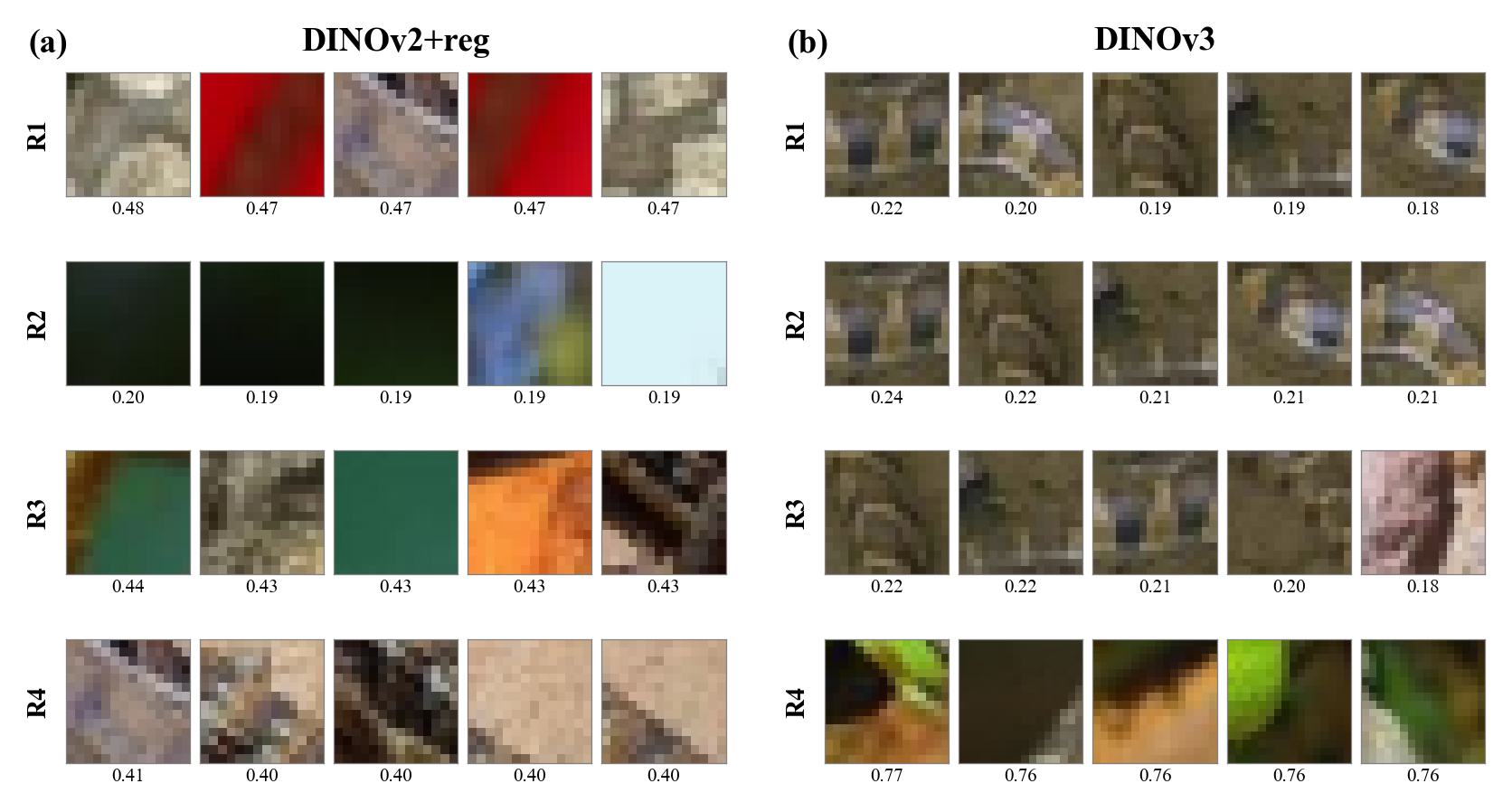
How to read this gallery: Higher cosine similarity means a patch more closely matches the register’s learned representation. In DINOv2+reg, try R2 — all 5 nearest neighbors are dark, low-information patches (cos ~0.20), confirming its role as an artifact absorber. R1/R3/R4 show more diverse, semantically meaningful patches at higher similarity (~0.47). In DINOv3, R4 stands out with strong matches to green vegetation textures (cos ~0.77) — a clear texture specialist. R1/R2/R3 all weakly match earthy ground patches (cos ~0.2), suggesting they don’t specialize on any specific visual pattern. But don’t confuse visual similarity with semantic content: DINOv3’s R3 carries the most classification information (50.1% probe accuracy) despite not resembling any specific patch type. It encodes abstract semantics, not visual templates.
When Do Registers Become Important?
This is the mechanistic core of our work. We traced two signals across all 12 transformer layers: attention routing (how much attention mass flows to registers) and semantic content (how much classification information each register carries). These turn out to be dissociated.
CLS attention distribution
Before looking at per-layer dynamics, here’s the high-level picture: how does CLS distribute its attention across token types?

Explore the actual CLS and register attention maps across different images. Toggle between CLS attention (where the CLS token looks) and register attention (where registers collectively attend):
Interactive: Attention map overlays
Attention flow across layers
We computed the mean attention weights across 200 ImageNet images, decomposing each layer’s attention into 9 source→target flows (CLS, registers, patches, each attending to each).
Interactive: Attention flow across layers
Use the slider to see how attention mass redistributes across layers. Watch how patches progressively attend more to registers in DINOv3.
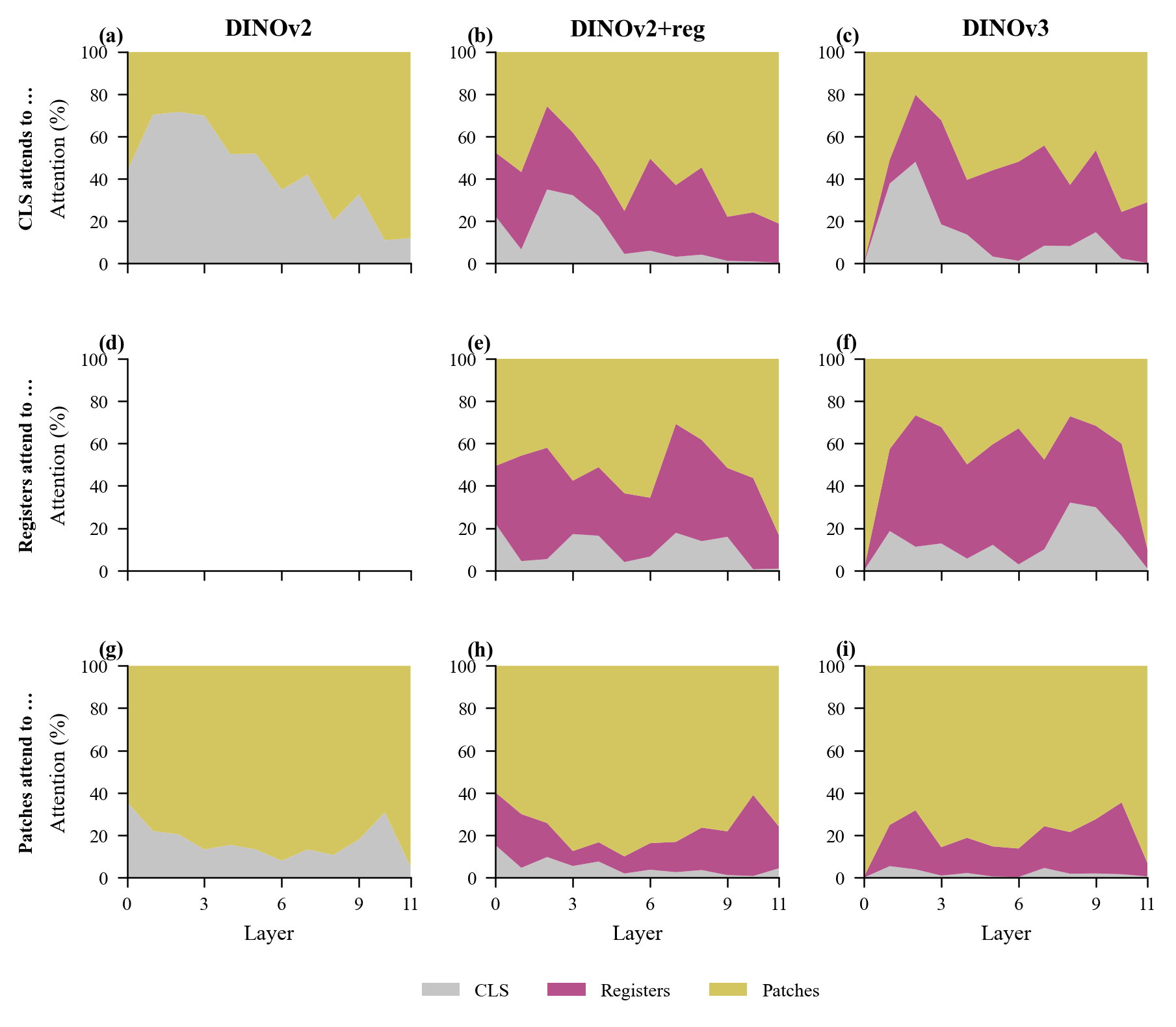
Key observations:
- DINOv2 (no registers): CLS receives 20–36% of patch attention throughout, serving as the sole global aggregation point.
- DINOv2+reg: Registers receive up to 17.9% of CLS attention, concentrated in R2 (16.1%). Registers are subordinate to CLS.
- DINOv3: Register attention builds gradually from mid-layers, reaching 28.7% of total patch attention by layer 11. R1 alone captures 21.1%. Registers become a major computational pathway.
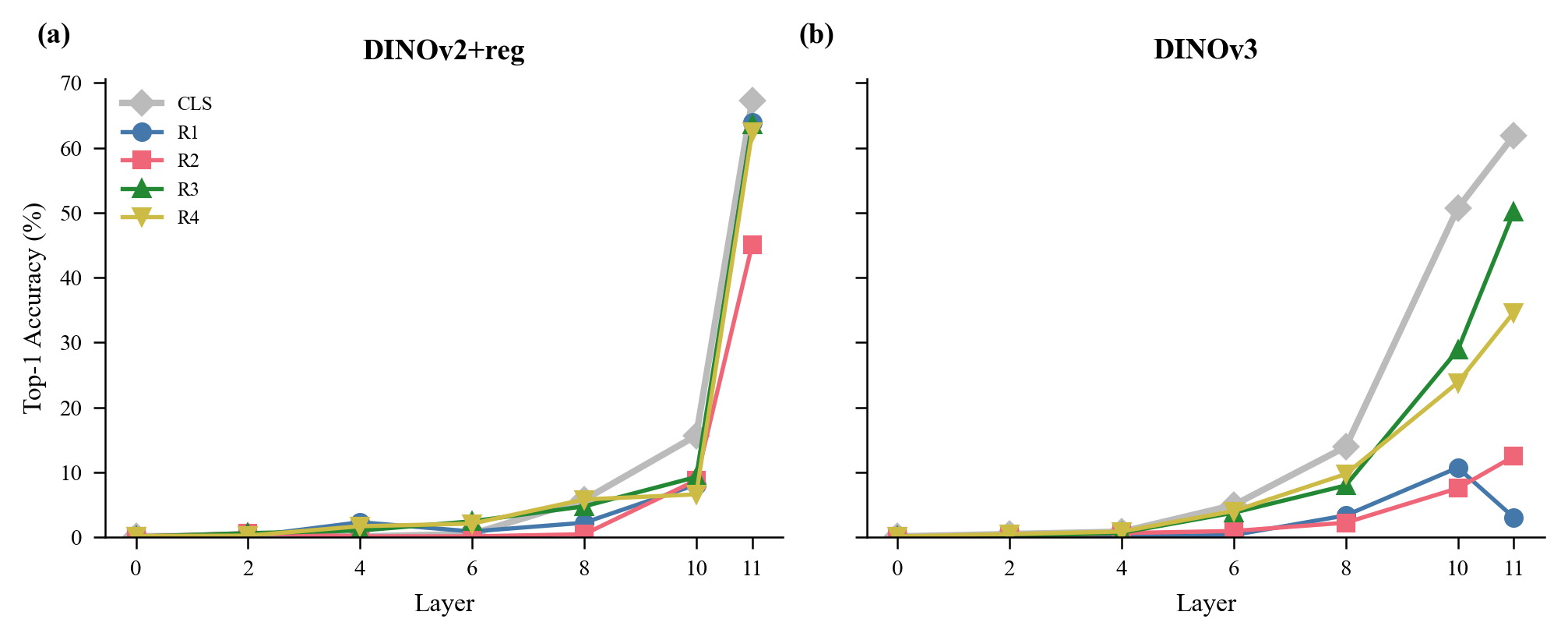
Layer-wise probing: when does semantic content emerge?
We trained linear probes on each register’s embedding at 7 intermediate layers (0, 2, 4, 6, 8, 10, 11) to track when classification information appears.
Interactive: Layer-wise register probing
Drag the slider to see classification accuracy at each layer. Note the explosive emergence at layers 10–11 and the transient R1 peak in DINOv3.
Layer-wise task performance
The layer sweep tells a complementary story: how does task performance (not just register probing) evolve across layers?

The temporal dissociation
The attention and probing data reveal a fundamental dissociation:
- Attention routing builds gradually: Patches start attending to registers from mid-layers onward, ramping smoothly.
- Semantic content emerges abruptly: All tokens carry near-random classification accuracy through layer 8 (< 6% for DINOv2+reg, < 14% for DINOv3). Then at layers 10–11, accuracy explodes — CLS jumps to 67.3%/61.9%, and specific registers follow.
These two signals are temporally dissociated: the attention routing infrastructure is built several layers before any semantic content appears. Registers are being used as computation targets before they carry meaningful information.
Even more striking are the per-register dynamics:
- DINOv3 R1: Peaks at layer 10 (10.7% accuracy) then drops to 3.0% at layer 11 — despite receiving the most attention (21.1%). R1 appears to be a transient computation buffer that processes information and releases it.
- DINOv3 R3: Progressively accumulates from 28.9% (layer 10) to 50.1% (layer 11) — a semantic accumulator.
- DINOv2+reg R1/R3/R4: All acquire and retain classification information (61–64% at layer 11) — semantic endpoints.
This suggests registers serve dynamic computational roles that change across layers, not fixed storage functions.
Cumulative vs. Individual Register Effects
When we zero registers one at a time, the effects are modest — but they reveal which registers matter most for which tasks.

But zeroing all four together produces a collapse far exceeding the sum of individual effects:
- DINOv2+reg: Sum of individual G1 deltas = −5.2pp, collective = −18.9pp
- DINOv3: Sum of individual = −7.0pp, collective = −36.6pp
This non-additive interaction confirms that registers function as a coordinated system. Their value lies not in what any single register contributes, but in the collective attention scaffold they provide.

Does This Scale? Controls and Validation
ViT-S vs ViT-B
We replicated all key experiments with ViT-B backbones. The ablation patterns are strikingly consistent across scales.

Is register zeroing special?
A natural concern: maybe zeroing any set of 4 tokens would be equally disruptive? We controlled for this by zeroing 4 randomly selected patch tokens instead of registers.

Practical Takeaways
Our findings have concrete implications for practitioners working with DINOv2 and DINOv3 features:
Don’t discard registers. If your pipeline extracts features from register-equipped models, include register tokens in your feature set. They are not auxiliary — they are load-bearing.
Mean substitution works as a fallback. If you must replace register values (e.g., for batching across models with different register counts), substituting dataset-mean activations preserves the attention scaffold and maintains accuracy.
Register specialization is exploitable. DINOv2+reg’s R2 encodes low-level image statistics; DINOv3’s R3 concentrates semantic content. These can be selectively queried for different downstream tasks.
Registers are active, not passive. The temporal dissociation — attention routing precedes semantic emergence — means registers participate in computation, not just storage. This has implications for pruning, distillation, and architectural design.
Scale-consistent. All findings replicate across ViT-S and ViT-B backbones, suggesting these are fundamental properties of the architecture rather than scale-dependent phenomena.
Citation
@inproceedings{parodi2026cls,
  title={CLS and Register Token Ablations Reveal Asymmetric
         Information Flow in Vision Transformers},
  author={Parodi, Felipe and Segado, Melanie},
  booktitle={Proceedings of the HOW Workshop at CVPR},
  year={2026}
}